Vision Transformer Demo

Introduction

This notebook intends to demonstrate how to use a vanilla transformer encoder to do computer vision tasks. This model will be trained on the classic Fashion MNIST dataset, and the implementation follows the original ViT paper.

Data Setup

To start, lets get the necessary imports and data setup with a mapping from class names to class values.

import numpy as np
import pandas as pd
import matplotlib.pyplot as plt
import torch
import torch.nn as nn
from torchvision import datasets
from torchvision.transforms import ToTensor
import os
from torchvision.io import read_image
from rich.progress import Progress
from torch.utils.data import DataLoader
from torchvision.transforms import ToTensor
import math
from sklearn.metrics import classification_report, confusion_matrix, ConfusionMatrixDisplay
import plotly
import plotly.graph_objects as go
from IPython.display import Markdown
from tabulate import tabulate

torch.manual_seed(0)

# DATA
training_data = datasets.FashionMNIST(
    root="../data",
    train=True,
    download=True,
    transform=ToTensor()
)

test_data = datasets.FashionMNIST(
    root="../data",
    train=False,
    download=True,
    transform=ToTensor()
)
batch_size = 24
train_loader = DataLoader(training_data, batch_size=batch_size, shuffle=True)
test_loader = DataLoader(test_data, batch_size=batch_size, shuffle=True)

class_dict = {
    0: "Top",
    1: "Trouser",
    2: "Pullover",
    3: "Dress",
    4: "Coat",
    5: "Sandal",
    6: "Shirt",
    7: "Sneaker",
    8: "Bag",
    9: "Ankle Boot"
}

Define our model

Next we’ll define our model. The model will be a standard transformer encoder, but some tweaks need to be made to handle computer vision tasks. First we’ll need to create a position encoder, which was borrowed from a common implementation freely available based on the original transformer paper. For simplicity, we’ll also create a MLP block, which is a simple linear layer followed by a non-linear activation.

The implementation of a Vision Transformer requires these steps,

1. Project each image patch into an embedding space through an MLP
2. Add a new “classification token” to the input sequence, which is an embedding of all ones to start
   • This classification token will be transformed into an embedding containing the relevant information needed to determine the class of the image
3. Add position encodings to each patch
4. Feed the patches into the encoder, applying the attention mechanism and projections along the way
   • The attention is not masked as all patches need to be compared and referenced among one another
5. After passing through the transformer layers, the transformed classification token is then put through a 3 layer MLP that will then classify the sequence

Some utility functions and processing steps are added to simplify calling the model externally.

class PositionalEncoding(nn.Module):

    def __init__(self, d_model: int, dropout: float = 0.1, max_len: int = 5000):
        super().__init__()
        self.dropout = nn.Dropout(p=dropout)

        position = torch.arange(max_len).unsqueeze(1)
        div_term = torch.exp(torch.arange(0, d_model, 2) * (-math.log(10000.0) / d_model))
        pe = torch.zeros(max_len, 1, d_model)
        pe[:, 0, 0::2] = torch.sin(position * div_term)
        pe[:, 0, 1::2] = torch.cos(position * div_term)
        #pe = pe.unsqueeze(0).transpose(0, 1)
        pe = torch.squeeze(pe)
        self.register_buffer('pe', pe)

    def forward(self, x):
        """
        Arguments:
            x: Tensor, shape ``[seq_len, batch_size, embedding_dim]``
        """
        x = x + self.pe
        return self.dropout(x)

class LinearLayer(nn.Module):

    def __init__(self, in_size, out_size):
        super().__init__()
        self.linear = nn.Linear(in_size, out_size)
        self.act = nn.GELU()

    def forward(self, x):
        return self.act(self.linear(x))

class VisionTransformer(nn.Module):

    def __init__(self, token_size, embedding_size, n_layers, n_classes):
        super().__init__()
        self.input_linear = nn.Linear(token_size, embedding_size)
        encoder_layer = nn.TransformerEncoderLayer(d_model=embedding_size, activation='gelu', batch_first=True, nhead=8, dim_feedforward=64)
        self.transformer_encoder = nn.TransformerEncoder(encoder_layer, num_layers=n_layers)
        mlp = [LinearLayer(embedding_size, embedding_size) for _ in range(3)]
        mlp.append(nn.Linear(embedding_size, n_classes))
        self.output_layer = nn.ModuleList(mlp)
        self.pe = PositionalEncoding(embedding_size, max_len=50)

    def __chip_image(self, image, chip_size=4):
        image_shape = torch.tensor(image.shape[-2:])
        num_chips = image_shape // chip_size
        chipped_out_images = torch.empty((*image.shape[:-2], int(torch.prod(num_chips).item()), chip_size, chip_size))
        count = 0
        for row in range(num_chips[0]):
            for col in range(num_chips[1]):
                r = row*chip_size
                c = col*chip_size
                chipped_out_images[:, :, count] = image[:, :, r:r+chip_size, c:c+chip_size]
                count += 1
        return chipped_out_images

    def forward(self, x):
        x = self.__chip_image(x).to(x.device)
        x = torch.squeeze(x.reshape((*x.shape[:3], -1)))
        x = self.input_linear(x)
        new_x = torch.ones(x.shape[0], x.shape[1]+1, x.shape[2], device=x.device)/5
        new_x[:, 1:] = x
        x = new_x
        x = self.pe(x)
        x = self.transformer_encoder(x)
        for layer in self.output_layer:
            x = layer(x)
        return x[:, 0]

Training

Training the model involves a standard training setup. Here are the hyperparameters,

• Number of Epochs = 10
• Learning rate = 5e-4
• Embedding Dimension = 64
• Number of Attention Layers = 3
• Optimizer = Adam
• Loss function = Cross Entropy

num_epochs = 20
model = VisionTransformer(16, 64, 3, 10)
device = "cuda:0"
model = model.to(device)
criterion = nn.CrossEntropyLoss()
optimizer = torch.optim.Adam(model.parameters(), lr=5e-4)
print(f"Number of model parameters: {sum(p.numel() for p in model.parameters() if p.requires_grad)}")
train_losses = []
test_losses = []

with Progress() as prog:
    epoch_task = prog.add_task("[red] Epoch", total=num_epochs)
    for epoch in range(num_epochs):
        train_task = prog.add_task("[blue] Train", total=len(train_loader))
        test_task = prog.add_task("[green] Test", total=len(test_loader))
        train_loss = 0.0
        test_loss = 0.0
        train_count = 0
        test_count = 0
        for x, y in train_loader:
            x = x.to(device)
            y = y.to(device)
            optimizer.zero_grad()
            predictions = model(x)
            loss = criterion(predictions, y)
            loss.backward()
            optimizer.step()
            train_loss += loss.item()
            train_count += x.shape[0]
            prog.update(train_task, advance=1, description=f"[blue] Train Loss: {train_loss/train_count:.3e}")
        train_losses.append(train_loss/train_count)
        with torch.no_grad():
            for x, y in test_loader:
                x = x.to(device)
                y = y.to(device)
                predictions = model(x)
                loss = criterion(predictions, y)
                test_loss += loss.item()
                test_count += x.shape[0]
                prog.update(test_task, advance=1, description=f"[green] Test Loss: {test_loss/test_count:.3e}")
        test_losses.append(test_loss/test_count)

        prog.remove_task(train_task)
        prog.remove_task(test_task)
        prog.update(epoch_task, advance=1)

/home/jon/projects/ml_demos/ml_demos/demos/venv/lib/python3.13/site-packages/rich/live.py:231: UserWarning:

install "ipywidgets" for Jupyter support

/home/jon/projects/ml_demos/ml_demos/demos/venv/lib/python3.13/site-packages/torch/nn/modules/linear.py:125: 
UserWarning:

Attempting to use hipBLASLt on an unsupported architecture! Overriding blas backend to hipblas (Triggered 
internally at /pytorch/aten/src/ATen/Context.cpp:310.)

Number of model parameters: 89866

Evaluate the model

Evaluating the model can proceed in several steps. First we can look at the loss plot to hint at model convergence. Here we can see the train and test loss values follow one another well. It does seem to indicate that at around epoch 7, overfitting may begin as the lines begin to diverge. The train loss is still trending downwards, while the test loss seem to have approached an asymptote.

epochs = [i for i in range(num_epochs)]
fig = go.Figure()
fig.add_trace(go.Scatter(x=epochs, y=train_losses, mode="lines+markers", name="Train"))
fig.add_trace(go.Scatter(x=epochs, y=test_losses, mode="lines+markers", name="Test"))
fig.update_xaxes(title_text="Epoch")
fig.update_yaxes(title_text="Loss")
fig.show()
predictions = []
truth = []
with torch.no_grad():
    for x, y in test_loader:
        x = x.to(device)
        p = model(x)
        preds = torch.argmax(p, dim=1)
        predictions.extend(preds.flatten().cpu())
        truth.extend(y)

Next lets look at the classic classification metrics of: Precision, Recall and F1

Markdown(tabulate(pd.DataFrame(classification_report(truth, predictions, target_names=class_dict.values(), output_dict=True)).transpose(), headers=["Class", "Precision", "Recall", "F1", "Support"]))

Class	Precision	Recall	F1	Support
Top	0.800382	0.838	0.818759	1000
Trouser	0.985729	0.967	0.976275	1000
Pullover	0.758459	0.807	0.781977	1000
Dress	0.826715	0.916	0.86907	1000
Coat	0.784536	0.761	0.772589	1000
Sandal	0.971904	0.934	0.952575	1000
Shirt	0.709288	0.588	0.642974	1000
Sneaker	0.928641	0.95	0.939199	1000
Bag	0.964036	0.965	0.964518	1000
Ankle Boot	0.941929	0.957	0.949405	1000
accuracy	0.8683	0.8683	0.8683	0.8683
macro avg	0.867162	0.8683	0.866734	10000
weighted avg	0.867162	0.8683	0.866734	10000

Overall the metrics indicate that the model is performing fairly reasonably. Most of the classes have F1 scores 0.75 or more. The classes that seemed to struggle more were,

1. Shirt
2. Pullover
3. Coat

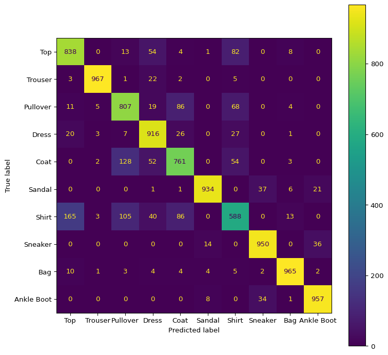
Intriguing that these were the lower performing classes, as these classes are similar to one another conceptually and visually. To determine if the model is indeed confusing these classes, the confusion matrix may provide more insight.

fig, ax = plt.subplots(figsize=(9, 9))
ConfusionMatrixDisplay.from_predictions(truth, predictions, display_labels=class_dict.values(), ax=ax)
plt.show()

The confusion matrix does indeed seem to allude to the idea that the model is confusing the three classes with one another. We can see that the largest off-diagonal values in the confusion matrix are these values intersections.

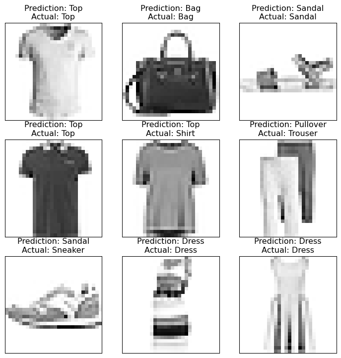
Finally let’s grab a few random samples from the test set and visualize them with the models predictions vs the truth values.

num_samples = 9
fig, ax = plt.subplots(3, 3, figsize=(9, 9))
test_sample = next(iter(test_loader))[:num_samples]
test_predictions = torch.argmax(model(test_sample[0].to(device)), dim=1)
row = 0
col = 0
for i in range(num_samples):
    ax[row, col].imshow(test_sample[0][i][0], cmap="Greys")
    ax[row, col].set_title(f"Prediction: {class_dict[int(test_predictions[i])]}\nActual: {class_dict[int(test_sample[1][i])]}")
    ax[row, col].set_xticks([])
    ax[row, col].set_yticks([])  
    col += 1
    if col > 2:
        row += 1
        col = 0
#plt.savefig("test_examples.png")
plt.show()