This notebook intends to demonstrate how to use a basic CNN to solve a computer vision task. This model will be trained on the classic Fashion MNIST dataset, and the implementation is just a simple CNN based on the successful pattern shown in AlexNet.
Data Setup
To start, lets get the necessary imports and data setup with a mapping from class names to class values. Luckily for us, this dataset is already normalized and split into train and test sets, allowing for quick prototyping.
Next we’ll define our model. The model is a simple CNN that will work to extract features from the input image. Each convolutional block will extract a higher order latent feature set from the input feature set. This will continue for several layers until the final latent representation is flattened and a standard ANN is applied to do a standard classification prediction.
Code
class LinearLayer(nn.Module):def__init__(self, in_size, out_size):super().__init__()self.linear = nn.Linear(in_size, out_size)self.act = nn.GELU()def forward(self, x):returnself.act(self.linear(x))class MyCNN(nn.Module):def__init__(self, input_channels=1, kernel_size=3, stride=1, n_classes=10):super().__init__()self.conv1 = nn.Conv2d(input_channels, 3, kernel_size=kernel_size, stride=stride, padding='same')self.conv2 = nn.Conv2d(3, 6, kernel_size=kernel_size, stride=stride, padding='same')self.pool = nn.MaxPool2d(kernel_size=2)self.projection = LinearLayer(294, 64) mlp = [LinearLayer(64, 64) for _ inrange(3)] mlp.append(nn.Linear(64, n_classes))self.output_layer = nn.ModuleList(mlp)def forward(self, x): batch_size, channels, height, width = x.shape x =self.conv1(x) x =self.pool(x) x =self.conv2(x) x =self.pool(x) x = x.reshape(batch_size, -1) x =self.projection(x)for layer inself.output_layer: x = layer(x)return x
Training
Training the model involves a standard training setup. Here are the hyperparameters,
Number of Epochs = 20
Learning rate = 1e-3
Optimizer = Adam
Loss function = Cross Entropy
Code
num_epochs =20model = MyCNN()device ="cuda:0"model = model.to(device)criterion = nn.CrossEntropyLoss()optimizer = torch.optim.Adam(model.parameters(), lr=1e-3)print(f"Number of model parameters: {sum(p.numel() for p in model.parameters() if p.requires_grad)}")train_losses = []test_losses = []model_states = []with Progress() as prog: epoch_task = prog.add_task("[red] Epoch", total=num_epochs)for epoch inrange(num_epochs): train_task = prog.add_task("[blue] Train", total=len(train_loader)) test_task = prog.add_task("[green] Test", total=len(test_loader)) train_loss =0.0 test_loss =0.0 train_count =0 test_count =0for x, y in train_loader: x = x.to(device) y = y.to(device) optimizer.zero_grad() predictions = model(x) loss = criterion(predictions, y) loss.backward() optimizer.step() train_loss += loss.item() train_count += x.shape[0] prog.update(train_task, advance=1, description=f"[blue] Train Loss: {train_loss/train_count:.3e}") train_losses.append(train_loss/train_count)with torch.no_grad():for x, y in test_loader: x = x.to(device) y = y.to(device) predictions = model(x) loss = criterion(predictions, y) test_loss += loss.item() test_count += x.shape[0] prog.update(test_task, advance=1, description=f"[green] Test Loss: {test_loss/test_count:.3e}") test_losses.append(test_loss/test_count) prog.remove_task(train_task) prog.remove_task(test_task) prog.update(epoch_task, advance=1) model_states.append(model.state_dict())
/home/jon/projects/ml_demos/ml_demos/demos/venv/lib/python3.13/site-packages/rich/live.py:231: UserWarning:

install "ipywidgets" for Jupyter support
/home/jon/projects/ml_demos/ml_demos/demos/venv/lib/python3.13/site-packages/torch/nn/modules/linear.py:125:
UserWarning:

Attempting to use hipBLASLt on an unsupported architecture! Overriding blas backend to hipblas (Triggered
internally at /pytorch/aten/src/ATen/Context.cpp:310.)
Number of model parameters: 32208
Evaluate the model
Evaluating the model can proceed in several steps. First we can look at the loss plot to hint at model convergence. Here we can see the train and test loss values diverge quite quickly, after only epoch 3. The model continues to improve the loss with the training set, while the test set continues to hover and even increase as the epochs continue. This indicates textbook overfitting, where the model is optimizing across some hyper specific features to the train set that don’t generalize well, The model state with the lowest test loss, biased to the epoch with a similar train loss should be selected as the best generalized model. Let’s select the model state at epoch 3.
Code
epochs = [i for i inrange(num_epochs)]fig = go.Figure()fig.add_trace(go.Scatter(x=epochs, y=train_losses, mode="lines+markers", name="Train"))fig.add_trace(go.Scatter(x=epochs, y=test_losses, mode="lines+markers", name="Test"))fig.update_xaxes(title_text="Epoch")fig.update_yaxes(title_text="Loss")fig.show()predictions = []truth = []best_model = model_states[3]model.load_state_dict(best_model)model.eval()with torch.no_grad():for x, y in test_loader: x = x.to(device) p = model(x) preds = torch.argmax(p, dim=1) predictions.extend(preds.flatten().cpu()) truth.extend(y)
Next lets look at the classic classification metrics of: Precision, Recall and F1
Overall the metrics indicate that the model is performing fairly reasonably. Most of the classes have F1 scores 0.8 or more, with a notable exception with the shirt class. The classes that seemed to struggle more were,
Shirt
Pullover
Coat
Top
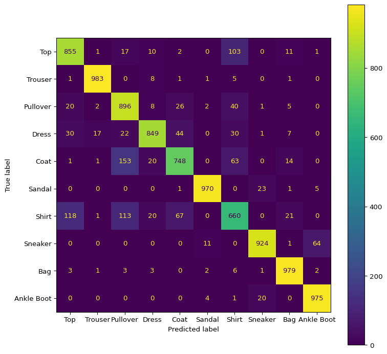
Intriguing that these were the lower performing classes, as these classes are similar to one another conceptually and visually. To determine if the model is indeed confusing these classes, the confusion matrix may provide more insight.
The confusion matrix does indeed seem to allude to the idea that the model is confusing the three classes with one another. We can see that the largest off-diagonal values in the confusion matrix are these values intersections.
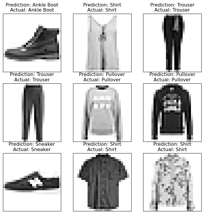
Finally let’s grab a few random samples from the test set and visualize them with the models predictions vs the truth values.
Code
num_samples =9fig, ax = plt.subplots(3, 3, figsize=(9, 9))test_sample =next(iter(test_loader))[:num_samples]test_predictions = torch.argmax(model(test_sample[0].to(device)), dim=1)row =0col =0for i inrange(num_samples): ax[row, col].imshow(test_sample[0][i][0], cmap="Greys") ax[row, col].set_title(f"Prediction: {class_dict[int(test_predictions[i])]}\nActual: {class_dict[int(test_sample[1][i])]}") ax[row, col].set_xticks([]) ax[row, col].set_yticks([]) col +=1if col >2: row +=1 col =0plt.show()